
Excel is a great tool to manage and analyze your data, it (almost) doesn’t matter how much data you have. When you need a strong tool to handle and organize your account, Excel is your best friend. Today, I’m gonna show you 5 great excel functions every PPC ninja needs to master. Hold tight Grasshoppers, here we go.
1. Use SUBSTITUTE and CONCATENATE (or just &) to Turn Broad Keywords into Broad Match Modified Keywords
The SUBSTITUTE formula works just like find and replace. It lets you search for a specific character or set of characters and replaces it with others.
The CONCATENATE formula gathers characters or text from different cells. The “&” works the same way, but quicker!
So, in order to turn broad keywords from column A into BMM keywords, we’ll start by adding a plus sign (+) before the keyword:
=”+”&A2 .
But what if you’d like to use it with all of your keywords?
That’s where SUBSTITUTE comes to action. Use SUBSTITUTE to replace every space, with a space followed by a plus sign (turn ” ” into ” +”). It should look as follows:
=SUBSTITUTE(A2, ” “, ” +”).
And the whole thing together:
=”+”&SUBSTITUTE(A2, ” “, ” +”) and voila:

2. Use TRIM and LEN to Count Characters In Your Ad Copy, and IF to Make Sure That Everything’s In Order
It’s easy to go wrong when writing a lot of ads at once. One of the most common mistakes is the use of too many characters. The right way to do it is to count the characters of each part of the ad (after using TRIM to make sure there isn’t any unnecessary spaces), and then we’ll see how IF can be used easily to make sure the ad meets all the requirements.
=LEN(TRIM(A2)) will count the characters in A2, minus the spaces that are sometimes typed by mistake.

By using a combination of IF, LEN and TRIM, we get an output of “V” or “X” to indicate ads that can’t be uploaded to AdWords.
=IF(Len(TRIM(A2))>25,”X”, IF(LEN(TRIM(B2))>35,”X”, IF(LEN(TRIM(C2))>35,”X”, IF(LEN(TRIM(D2))>35, “X”, “V”)
The thing we’ve done here is to get an X in E2 if we exceeded the character limit (minus extra spaces) in any one of the fields, or get a V if everything is in the right length. If plan to copy and paste this formula, make sure to replace A2 with your Headline cell, since the headline is the only part of your ad which isn’t limited to 35 characters.
3. Use Pivot Table to Summarize Your Data
The best way to explain the need of this great Excel feature is by downloading a placement report on the account level. You can see for yourself that a big part of the placements appears more than once. In order to summarize the data and see the overall performance of each placement, we’ll use a Pivot Table.
Ninja Tip: Add to your Pivot Table only columns that can be summed. CTR, Avg Pos and conversion rate cannot be summed so it’s best to add (Sum of) Impressions, (Sum of) Clicks, (Sum of) Cost and (Sum of) Conversions and calculate the rest by yourself.
Don’t forget to add the column you want summarized in “Rows”.
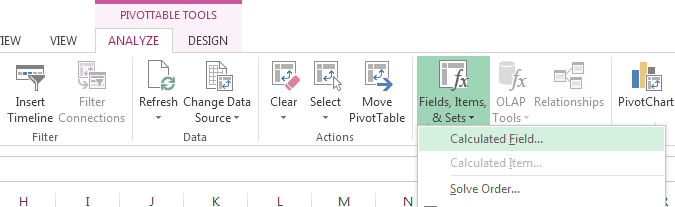
Ninja Tip 2: To calculate fields (like CTR for example), you have two options:
I. Add calculated fields by clicking here:
And then insert your formula
II. (My favorite): Copy the entire Pivot Table and paste it as values in a new spreadsheet, then insert your formulas and double click the bottom right part of the cell and BAM! It’s done.
4. Use VLOOKUP to Compare Data From AdWords And Data from your CRM or Other Traffic Sources.
VLOOKUP is a great way to organize your data for optimization. What it does is to look for a certain value (let’s say Placement for example), and returns its associated metrics (if you’re using a CRM system and passing the {placement} parameter in your URL, you’ll be able to see if leads coming from this placement turned into sales).
Let’s see how it’s done:
First, we’ll download all the data we need from AdWords and the CRM (make sure that you have the placement in both files, since you’ll use this column as the common ground between the two data sheets).
I like to add all the data into one spreadsheet, but it’s up to you – as you’re able to use VLOOKUP with more than 1 file.
What we’ll do here is to look for placements report and see if they’re in the Sales report from the CRM (it’s best to VLOOKUP after using Pivot table because it will save you a lot of time waiting for your computer to be done, but also, so you can get the number of sales coming from each placement [sum of sales]).
Download this spreadsheet, I made this one just for you to practice.
in F2 insert the following formula:
=VLOOKUP(A2, H:J,2,0)
A2 – is what we’re looking for
H:J – is the range in which we’re looking for A2
2 – Is the column number between H and J from which we’d like to get the value (2 is the 2nd column from the left – column I)
0 – means that we want Excel to find the exact text found in A2, and not find the closest.
Now, try to calculate the ROI for each placement by using VLOOKUP.
Ninja Tip: You can also use VLOOKUP to compare a keyword (or placement’s) data from all time and last 14 (or last 30) to see if it still works as well.
5. Polish Your Ads with PROPER, LOWER or UPPER
The last trick is pretty simple. And yet, can save you a lot of time and headaches. By using the PROPER command, you can change your text capitalization in seconds!
PROPPER will capitalize the first letter of every word.
LOWER will make sure that nothing is capitalized .
and UPPER will make every letter capitalized (not recommended for ads creative, but I trust that you’ll find a good use for it).
6. Bonus: Use Heat Maps To See Hour By Hour Trends In Your AdWords Account
Check out this awesome post by Daniel Gilbert, Thank me later 😉
That’s it for this time, if you have anything you want to ask or share, or if you think I forgot a cool Excel formula, use the comments below.
Cheers.
Follow @roydanino